Written by Debra Dalgleish from Contextures Blog
When you create a pivot table in Excel, it doesn’t matter if there are filters applied in the source data table. The pivot table includes all the data, whether it’s hidden or not. But, if you’d like to create a pivot table from filtered list visible rows only, you can try this technique.
Excel Versions
This technique uses new features in Excel, that are found in Excel for Office 365. Be sure that your version of Excel has the new functions, such as SORT and UNIQUE. I don’t want you to waste your time trying something that won’t work for you!
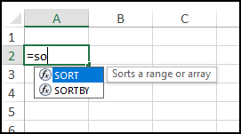
To check for the new functions:
- Select a blank cell, then type: =SO
- If the screen tip shows SORT and SORTBY, you have the new functions.
Named Excel Table
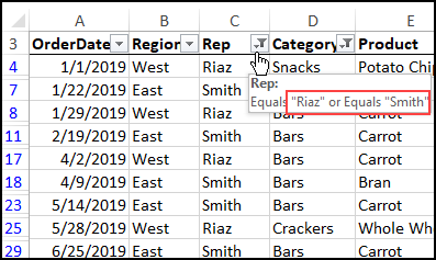
In this example, the source data that we want to use for the pivot table is a named Excel table — Sales_Data.
There are 100 records in the table, and it’s currently filtered to show 2 of the sales rep names (Smith and Riaz), and all of the categories except Cookies.
NOTE: If your pivot table source data has a huge number of records, the following technique could slow down your workbook
Make a Pivot Table
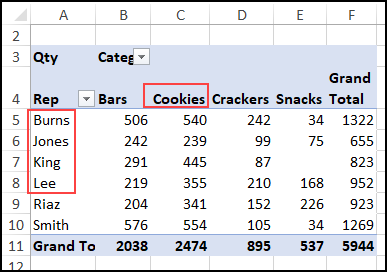
If I create a pivot table from the Sales_Data table, it will include all 100 records, not just the visible row records.
All the sales rep names are listed, and all the categories are included.
Pivot From Filtered List
To create a pivot table from filtered list visible rows only, I’ll do these steps:
- Add a new column in the Sales_Data table.
- In that column, use a formula to mark the visible rows
- On another sheet, get the source data headings
- Use a new function to pull visible rows from the Sales_Data table
- Create a dynamic named range, based on pulled data and headings
- Create a pivot table based on the dynamic named range
Mark the Visible Rows
The first step is to add a new column in the Sales_Data table, to mark the visible rows, using the SUBTOTAL function.
- In cell J3, type the heading – Vis
- In cell J4, start this SUBTOTAL formula, with 2 (Count) as the function number:
- =SUBTOTAL(2,
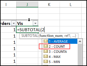
- Then, click on cell I4, which has the number of Orders, and type a closing bracket.
- =SUBTOTAL(2,[@Orders])
- Press Enter, to add the formula to all the cells in the Vis column (even the hidden rows)
How It Works
All the visible rows show 1 as the formula result in column J.
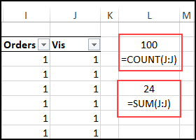
But, if you use formulas to do a COUNT and a SUM for column J, you’ll see that the numbers are different.
There are 100 numbers in column J, but only 24 of those numbers are a 1.
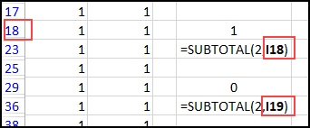
The SUBTOTAL function ignores values that are hidden by a filter (and manually hidden rows, in some cases), so for non-visible rows, the result in column J is zero. For example:
- row 18 is visible, so it returns a 1
- row 19, is hidden by the filter, so it returns a zero
Start a New Sheet
We’ll create a new worksheet, and build a new source for the pivot table there.
- Insert a new worksheet
- Name the sheet – DataFiltered
To build a pivot table, the data needs headings, so we’ll use the ones from the Sales_Data table.
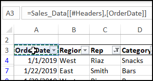
- In cell A1 on the new sheet, type an equal sign
- Go to the FoodSales sheet, and click on cell A3, which has the first heading cell in the Sales_Data table.
- Press Enter, to complete the formula
Next, follow these steps to get the rest of the headings
- Select cell A1, which has the link to the first heading
- Point to the fill handle, at the bottom right corner of cell A1
- Drag across to column J, to get the rest of the Sales_Data table headings
- (optional) Format the heading cells in bold font
Get the Filtered Data
Next, we’ll use a new Excel function — FILTER — to pull the visible rows from the Sales_Data table
- Select cell A2, and start the formula:
=FILTER(
The first argument is the array – what we want to filter.
Type the name of the table that we want to filter – Sales_Data, then type a comma
=FILTER(Sales_Data,
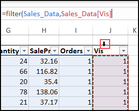
The next argument is include – our rule for which records to return in the results. We want the rows where there is a 1 in the Vis column.
- Go to the FoodSales sheet, and click at the top of the Vis column heading cell
- The table name and column name are added to the formula
=FILTER(Sales_Data,Sales_Data[Vis]
- Type our rule for that column: =1
=FILTER(Sales_Data,Sales_Data[Vis]=1
- Type a closing bracket, then press Enter to complete the formula

Dynamic Array of Filtered Data
Even though you only entered the formula in cell A2, the formula results are in a dynamic array, that spills down and across, in as many cells as needed.
There is a thin blue border around the dynamic array
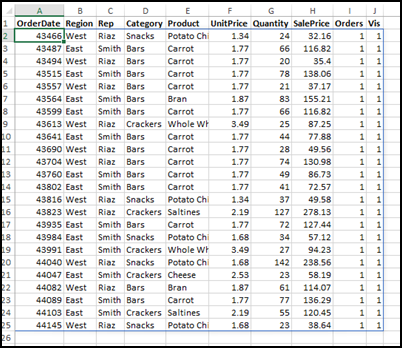
Cells in the Dynamic Array
If you click in any cell in the dynamic array, other than cell A2,
- you can see the formula in light grey font in the formula bar
- you can’t make any changes to the formula
If you select cell A2, where the formula was entered, you can edit the formula, as usual
Create a Dynamic Named Range
Now that we have headings and filtered data, we’ll create a dynamic named
range to use as the pivot table’s source data.
To refer to a dynamic array in a formula, use the array’s starting cell, followed by the spill operator – #
In this example, here’s the dynamic array reference:
DataFiltered!$A$2#
We’ll use that reference in an OFFSET formula, to create the dynamic range:
- On the Excel Ribbon, click the Formulas tab, then click the Define Name command
- For the Name, type: PivotUse
- Leave the Scope as Workbook
- In the Refers to box, enter this OFFSET formula:
=OFFSET(DataFiltered!$A$2#,-1,0, ROWS(DataFiltered!$A$2#)+1, COLUMNS(DataFiltered!$A$2#))
- Click OK, to complete the name
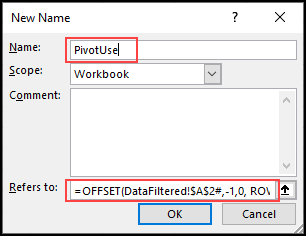
How the OFFSET Formula Works
The OFFSET function returns a range that:
- Starts at the dynamic array
- Goes up one row (-1)
- Moves over 0 columns
- Includes the number of rows in the dynamic array, plus 1 for the heading row
- Includes the number of columns in the dynamic array
If the filters on the Sales_Data table are changed, the number of rows in the dynamic array will change.
Our dynamic named range, PivotUse, will adjust to those changes automatically
Create the Pivot Table
The final step is to create a pivot table, based on the dynamic named range.
- Insert a new sheet, and name it PivotVis
- Select any cell on the new sheet
- On the Excel Ribbon, click the Insert tab
- Click the Pivot Table command
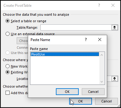
- In the Create PivotTable dialog box, click in the Table/Range box, and press the F3 key on your keyboard
- In the Paste Name list, click on PivotUse, and click OK
- For the location, choose the PivotVis sheet
- Click OK to create the pivot table.
Add Fields to the Pivot Table
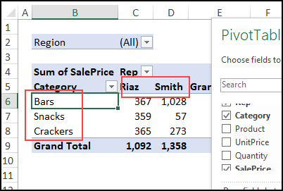
Next, use the PivotTable Field List to add the fields that you want to show in the pivot table.
If you include the Rep and Category fields, you’ll see that they only include the items from the visible rows in the Sales_Data table.
Change the Sales_Data Filters
If you change the filters in the Sales_Data table, be sure to refresh the pivot table after you’ve finished making the changes.
For example, filter the data so it only shows sales in the East region.
The dynamic array updates automatically, and now there are only 14 rows on that sheet.
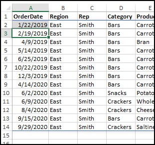
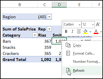
However, pivot tables don’t refresh automatically, so you can do that step manually.
Right-click on the pivot table, and click Refresh.
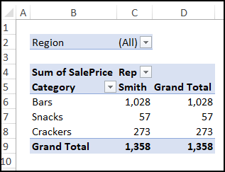
After the refresh, only the East region records are showing. Riaz didn’t make any sales in that region, so Smith is the only rep in the filtered data, and in the refreshed pivot table.
Get the Sample File
To see how the pivot table from filtered list visible rows technique works, go to the Pivot Table Source Data page on my Contextures site.
In the Download section, get the Filtered Source Data sample file. The zipped file is in xlsx format, and does not contain any macros.
__________________
More Pivot Table Info
How to Set Up an Excel Pivot Table
Pivot Table Dynamic Data Source
Create a Pivot Table in Excel
Macro to Filter Pivot Table Data
________________
Pivot Table from Filtered List Visible Rows

________________
Pivot Table from Filtered List Visible Rows is a post from Contextures Blog and is not allowed to be copied to other sites
