Go From 48672 Excel Formulas Down to 1

Happy Canada Day, if you’re celebrating tomorrow! And Happy July 4th, on Monday, if you’re in the USA! These holidays inspired me to change an Excel workbook, so it has a formula in only one cell. The old workbook needed 48,672 formulas, to do the same thing! Also, how often does Canada Day fall on a Friday? Let’s find out!

Country Flags in Excel

Way back in 2011, I showed you how to make flags in Excel, for Canada and the USA.

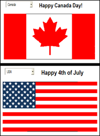
There’s a drop down list at the top left of the worksheet, where you can choose Canada, or USA.
Based on that selection, a message appears a the top centre of the sheet.
And, with a magical combination of:
- CHOOSE formulas
- Named ranges
- Conditional formatting
The selected country’s flag appears.

make country flags in Excel

Flag Workbook Setup

You can read all the details for setting up the flag workbook, but here’s a quick peek at how the flags are set up.

Note: To get the sample files, see the download section at the bottom of the page

In the Excel workbook, there are 2 flag sheets – Canada and USA.
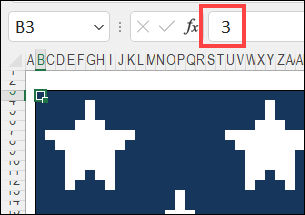
The close-up screen shot below shows the top left corner of the USA flag.

Rows and columns have been narrowed, to create tiny squares
Each cell has a number typed in it, as a colour code
- In the screen shot, cell B3 is selected
- It has a 3 entered in it – the code for the colour blue.
On the main sheet, CHOOSE formulas return the cell numbers from the selected country’s flag

Challenge: How many columns and rows are in the flag’s design?

Answer: See the next section.

colour code number in worksheet cell

What Are the Flag Dimensions?

So, what was your guess for the number of columns and rows in the flag’s design?

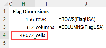
If you guessed 156 rows, and 312 columns, you were right!

And that is a total of 48,672 cells in each flag!

total number of cells in country flag

Flag Conditional Formatting

On the sheet with the Country selection drop down, there is another range, that is the same size as the Canada and USA flags.

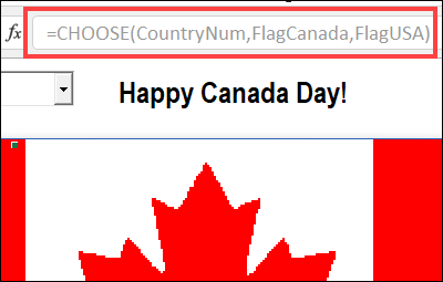
In the original version of the flag file, each of those 48,672 cells had a CHOOSE formula, which was array-entered for the entire range.

=CHOOSE(CountryNum,FlagCanada,FlagUSA)

The result in each cell was the colour code for the matching cell, in the selected country’s flag.

That’s a lot of formulas!

Flag Formulas for Excel 365

Looking at this workbook in 2022, I wondered if a single spill formula (available in Excel 365) could do the same job.

Tip: Go to my Contextures site for more Spill Function Examples

Here’s what I did, to find out if it was possible:

First, I selected all the cells with CHOOSE formulas, and cleared them
Next, I selected cell B3, and entered the CHOOSE formula in that cell only
To complete the formula, I pressed Enter
- It does NOT need to be array-entered, with Ctrl+Shift+Enter
The formula automatically spilled into the adjacent rows and columns, to complete the flag

That’s one formula cell, instead of 48,672 formula cells!

Check the Spill Formula Cells.

The formula is in only one cell now – cell B3.

If you select any other cell in the conditional formatting flag, the Formula Bar shows the formula, but you can’t edit it. It’s just a “spill” cell, not a formula cell.

For example, in the screen shot below:

Cell BT5 is selected
The dimmed out formula shows in the Formula Bar
If you click in the Formula Bar, the formula disappears – you can’t edit it

dimmed out formula in Excel formula bar

Question 2: Is It Friday Yet?

In a strange coincidence, Canada Day 2011 was on a Friday, just like it is this year, so both countries had a long weekend, at the same time.

How often does that happen? Excel helped me answer that question too!

First, in column A, I made a list of July 1st dates, starting in 1988.

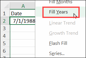
To do that, type 7/1/1988 in a cell
Select that cell, and point to the fill handle, at the bottom right corner of the cell
Press the right mouse button, and drag down, 30 or 40 rows
Release the mouse button, and click on Fill Years

Fill Years command

Get the Weekday Name

Next, I formatted the list of dates as a named Excel table.

After that, I added 3 more columns, with the following formulas:

First, in cell B1, B2 and B3, I typed the headings, Day, Row, Yrs
Next, in cell B2, I created a TEXT formula, to get the weekday name for each date.
- =TEXT(A2,”ddd”)
Then, in cell C2, I entered this formula, to get the row number for each Friday in the list:
- =IF(B2=”Fri”,ROW(),””)
Finally, to find the intervals between the Friday July 1st dates, I put this formula in cell D2:
- =IF(MAX(C$1:C1)=0,””, IF(C2=””,””, C2-MAX(C$1:C1)))

Filter the Canada Day List

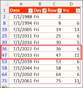
The final step was to filter the list, to show only the years that Canada Day falls on a Friday.

That makes it easy to see that the next occurrence is 11 years from now, in 2033. That’s a long time to wait!

And look at all the 11s in that pattern:

Occurrences are all 5, 6, or 11 years apart
Of course, 5 + 6 = 11
Occurs in 2011, 2022, 2033, 2044 (but not 2055)

I’m sure a math genius could explain the pattern, but I’m not one of those!

But at least I’m smart enough to create a custom Table Style, in a lovely shade of Canada Day red!

list of Canada Day Fridays

Get the Country Flag Files

To see how the Country Flag files work, you can go to the Excel Sample Files page on my Contextures site, and download them.

In the Conditional Formatting section, look for:

CF0013 – Canada and USA Flags – Original version, with NO spill formula
CF0014 – Canada and USA Flags (Excel 365) – New version, with spill formula

Both of the zipped files are in xlsx format, and there are no macros in either file.

_____________________