Learn how to crosshair highlight in excel, essentially, how to highlight row and column of active cell

Here’s how to achieve a crosshair cell highlighting effect where both row and column is highlighted where the cell is selected. This video will demonstrate how to quickly crosshair highlight active cell in Excel? Using excel to highlight active row and column conditional formatting is what I will be doing.

Here are the steps outlined in the video.

Highlight Selected Row
1) Ctrl + A
2) Home — Style — Conditional Formatting
3) New Rule
4) Select “Use a formula to determine which cells to format”.
5) =ROW()=CELL(“ROW”)
6) Format
7) Fill tab.
8) Select blue colour.
9) OK
10) OK

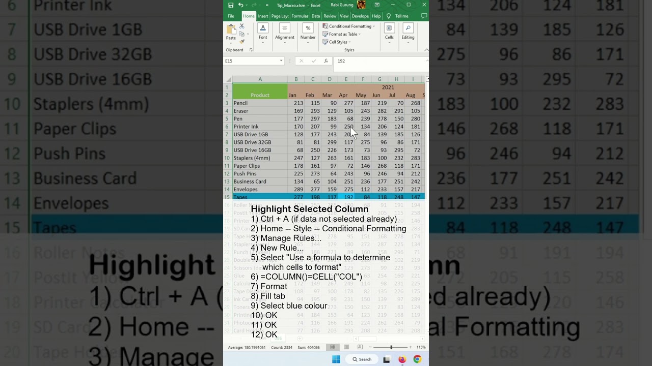
Highlight Selected Column
1) Ctrl + A (if dataset is not selected already)
2) Home — Style — Conditional Formatting
3) Manage Rules…
4) New Rule…
5) Select “Use a formula to determine which cells to format”.
6) =COLUMN()=CELL(“COL”)
7) Format
8) Fill tab.
9) Select blue colour.
10) OK
11) OK

Animation
1) Right-click sheet. View Code.
2) Select Worksheet
3) Enter these in Worksheet_SelectionChange()
Target.Calculate
4) Ctrl+S to save
5) Close Code Editor

Here are the past videos of how to create a crosshair highlight in Excel.

Crosshair Highlight With Intersecting Cell As Different Color – In Excel
https://youtube.com/shorts/dlgV0UCP0WU?feature=share

How to crosshair highlight enabled and disable in Excel – Excel Tips and Tricks
https://youtube.com/shorts/roOnmcbgbTI?feature=share

How to Enable and Disable Crosshair Highlight for Rows or Columns in Excel – Excel Tips and Tricks
https://youtube.com/shorts/l763DsFNFFU?feature=share

Crosshair highlight in Google Sheet – Excel Tips and Tricks
https://youtube.com/shorts/_bjYH4xVK5k?feature=share

#microsoft #excel #exceltips #tips #exceltricks #tricksandtips